Neural Networks And Deep Learning
Table of Contents
Introduction
Introduction to Deep Learning
A Neuron is inspired by the biological neuron and is the basic building block of neural networks. Neurons are responsible for computing and transmitting information through the network.
A neuron consists of a set of inputs, called dendrites, and a single output, called an axon. The inputs of a neuron are connected to the outputs of other neurons, forming a network of connections. Each connection is associated with a weight, which determines the strength of the connection.
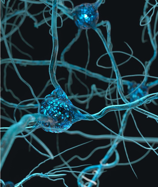
A biological neuron with its axon and dendrites.
Neural Networks are inspired by the human brain and they are comprised of node layers or neurons.
Each node or artificial neuron is connected to another neuron and has an associated weight and threshold. If the output of any individual neuron is above the specified threshold value, the neuron is activated, sending data to the next layer of the network. Otherwise no data is passed along to the next layer of the network.
Deep Learning is rising in recent times because of the amount of data available as well as the computational power provided. The other important factor is the development of even better deep learning algorithms and the invention of new more capable ones by the research community. 1
Neural Network Basics
Neural Network Basics
Logistic Regression as a Neural Network
In a Binary Classification problem, the result is a discrete value output - account hacked (1) or not hacked (0) - is a cat image (1) or a non-cat image (0).
Logistic Regression is an algorithm for Binary Classification, it estimates the probability of an event occurring, such as voted or didn’t vote, based on a given dataset of independent variables. Since the outcome is a probability, the dependent variable is bounded between 0 and 1. 𝐺𝑖𝑣𝑒𝑛 𝑥, 𝑦̂=𝑃(𝑦=1 | 𝑥), where 0 ≤𝑦̂≤1
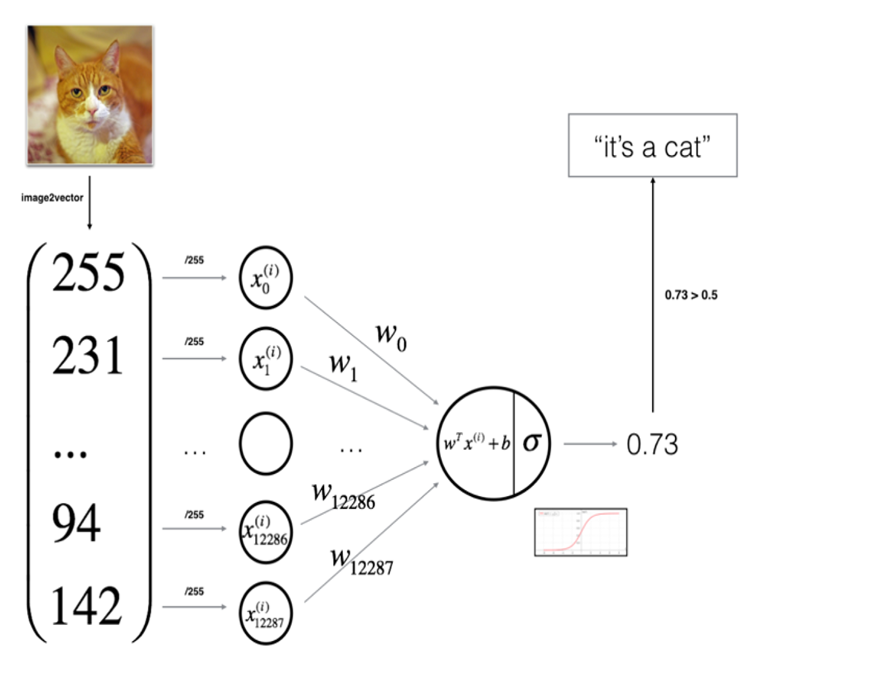
Logistic Regression consists of inputs, weights,
    logistic regression function and the activation function
In deep neural networks, the letter “z” is often used to represent the output of the linear combination of the weights and inputs at a particular layer in the network. This is also known as the pre-activation value or the weighted sum of the inputs.
For example, if we have a layer in a neural network with weights w and inputs x, the pre-activation value z for that layer can be calculated as follows:
z = w * x
The value of z is then passed through an activation function, which is a non-linear function that transforms the linear combination of the inputs and weights into a non-linear output. The activation function is typically applied element-wise to the value of z.
In summary, the letter “z” is used to represent the output of the linear combination of the weights and inputs at a particular layer in a neural network, before the activation function is applied.
The loss function measures the discrepancy between the prediction (𝑦̂(𝑖)) and the desired output (𝑦(𝑖)). In other words, the loss function computes the error for a single training example.
The cost function is the average of the loss function of the entire training set. We are going to find the parameters 𝑤 𝑎𝑛𝑑 𝑏 that minimize the overall cost function.
A Computation Graph is a visual representation of the operations performed by a computer program, especially a machine learning or deep learning model.
Vectorization is the process of converting a set of scalar values, or a sequence of operations, into a vector or a matrix.
In Python, broadcasting is a mechanism that allows arrays of different shapes to be used together in mathematical operations.
Normalization is the process of scaling a set of values to have a mean of 0 and a standard deviation of 1.
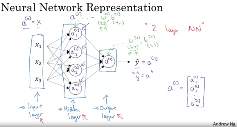
A shallow neural network consists of an input, a hidden and an output layer.
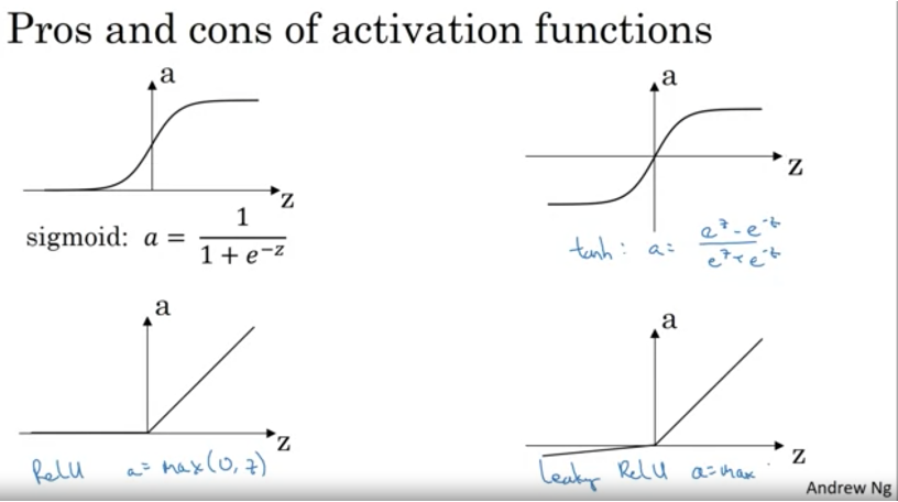
Activation functions are mathematical equations that determine the output of a neuron in a neural network.
Activation functions are used in artificial neural networks to introduce non-linearity into the model.
The sigmoid function, tanh function, and ReLU (rectified linear unit) function are all commonly used activation functions in neural network models.
The sigmoid function maps any input to a value between 0 and 1, which makes it a useful activation function for output layers that need to predict probabilities. However, the sigmoid function can saturate (i.e., produce output values that are very close to 0 or 1) when the input is large, which can slow down the training process and limit the model’s ability to learn.
The tanh function is similar to the sigmoid function, but it maps inputs to values between -1 and 1. Like the sigmoid function, the tanh function can saturate when the input is large, but it tends to perform better than the sigmoid function in certain scenarios.
The ReLU function is defined as f(x) = max(0, x), where x is the input. The ReLU function maps negative values to 0 and positive values to themselves, which makes it a more efficient activation function than the sigmoid and tanh functions. However, the ReLU function can produce “dying ReLU” units, which are units that produce output values of 0 for all inputs and do not contribute to the model’s prediction.
The leaky ReLU function is a variant of the ReLU function that addresses the issue of dying ReLU units by allowing a small negative slope (i.e., a “leak”) for negative input values. This helps to prevent the issue of dying ReLU units and can improve the model’s performance.
In summary, the sigmoid function is useful for output layers that need to predict probabilities, but it can be slow to train and prone to saturation. The tanh function is similar to the sigmoid function, but it tends to perform better in certain scenarios. The ReLU function is efficient but can produce dying ReLU units. The leaky ReLU function is a variant of the ReLU function that helps to prevent the issue of dying ReLU units.
Shallow Neural Networks
Shallow Neural Networks
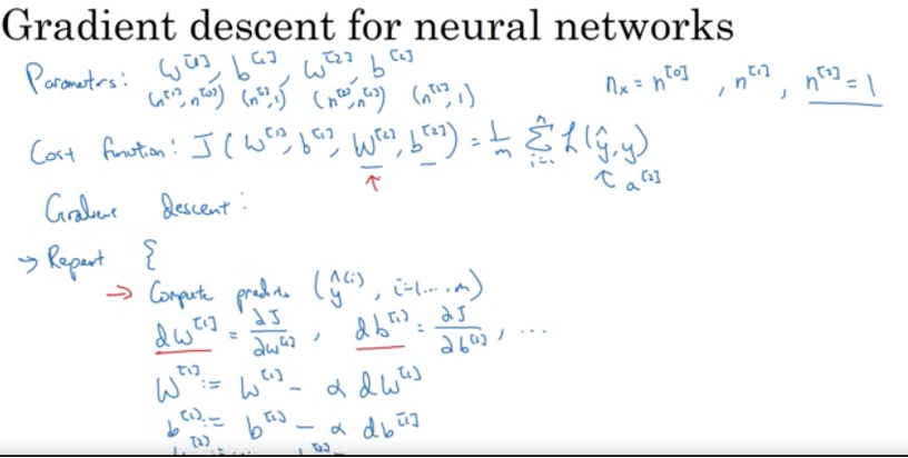
Gradient Descent is an optimization algorithm. The algorithm works by iteratively updating the values of the parameters in the direction that reduces the loss.
In gradient descent for deep neural networks, the values “w” and “b” are the weights and biases for the network, respectively. These values are updated during the training process to minimize the loss function of the network, which measures the difference between the predicted output and the true output for a given input.
The weights “w” represent the strength of the connection between the neurons in different layers of the network. They determine how much each input contributes to the output of the network. The biases “b” represent an additional parameter that can be adjusted to shift the output of the network up or down.
The intuition behind the weights and biases is that they allow the network to learn and make predictions based on the input data. The training process adjusts the values of the weights and biases to reduce the loss and improve the accuracy of the predictions made by the network.
In summary, the values “w” and “b” in gradient descent for deep neural networks are the weights and biases of the network, respectively. They are updated during the training process to minimize the loss function and improve the accuracy of the network’s predictions.
In gradient descent for deep neural networks, the values “dw” and “db” are the partial derivatives of the loss function with respect to the weights and biases, respectively. These values are used to update the weights and biases during the training process in order to minimize the loss function and improve the accuracy of the network’s predictions.
The partial derivative “dw” represents the change in the loss function with respect to a change in the weights “w”. It measures how much the loss function would change if the weights were adjusted by a small amount. The partial derivative “db” represents the change in the loss function with respect to a change in the biases “b”. It measures how much the loss function would change if the biases were adjusted by a small amount.
The intuition behind the partial derivatives “dw” and “db” is that they allow the network to learn and make predictions based on the input data. The training process adjusts the values of the weights and biases based on the partial derivatives in order to reduce the loss and improve the accuracy of the predictions made by the network.
In summary, the values “dw” and “db” in gradient descent for deep neural networks are the partial derivatives of the loss function with respect to the weights and biases, respectively. They are used to update the weights and biases during the training process in order to minimize the loss function and improve the accuracy of the network’s predictions.
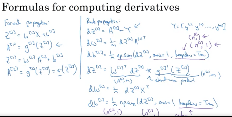
In Forward propagation the input data is processed through the network layers to generate output. Backpropagation’s goal is to adjust the weights of the connections in such a way as to minimize the difference between the predicted output of the network and the target output. A neural network in contrast with logistic regression that initializes its parameters with zero, has to randomly initialize its parameters in order to work.
A partial derivative is a derivative taken with respect to one variable, holding the other variables fixed. It allows you to see how much a function changes when you change one of its variables, while keeping the others constant.
For example, consider a function f(x,y) that depends on two variables x and y. The partial derivative of f with respect to x is denoted as ∂f/∂x, and it represents the rate of change of f with respect to x, holding y constant.
Similarly, the partial derivative of f with respect to y is denoted as ∂f/∂y, and it represents the rate of change of f with respect to y, holding x constant.
Partial derivatives are often used in multivariate calculus and are a fundamental tool for understanding how functions of multiple variables behave. They are used in a wide range of applications, including optimization, engineering, and economics.
In the context of mathematics and computer science, the term “convergence” typically refers to the process of approaching a specific value or set of values as a function of some variable.
For example, if a sequence of numbers is said to converge to a particular value, it means that as the numbers in the sequence get further and further along, they get closer and closer to the specified value. Similarly, if an iterative algorithm is said to converge, it means that as the algorithm progresses through its iterations, the output or result of the algorithm approaches a specific value or set of values.
In general, the concept of convergence is important in many areas of mathematics and computer science, as it allows us to understand how various processes and algorithms behave as they approach a specific result or set of results.
Convergence is often used to analyze the behavior of algorithms and other processes, and to understand how they perform as they approach a specific result or set of results.
Deep Neural Networks
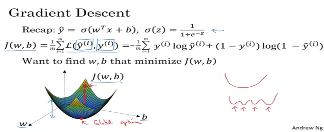
Gradient Descent is an optimization algorithm that is used to find the values of the weights and biases that minimize the loss function in a machine learning model. It involves adjusting the values of the weights and biases in small increments based on the gradient of the loss function until the loss is minimized or the model has reached a satisfactory level of performance.
Gradient descent is an optimization algorithm that is used to find the values of parameters (such as weights and biases) that minimize a loss function. It is a key part of the training process for many machine learning models, including neural networks.
In gradient descent, the model makes predictions based on a set of input data and compares the predictions to the true values (also known as the labels). The difference between the predictions and the true values is the loss, which is a measure of how well the model is performing. The goal of gradient descent is to find the values of the model’s parameters that minimize the loss.
Weights and biases are model parameters that are used to make predictions. In a neural network, weights are the values that are multiplied by the input data and summed together to produce the input for the activation function. Biases are added to the weighted sum of the inputs and can help the model make predictions that are shifted away from 0.
During the training process, the model uses gradient descent to adjust the values of the weights and biases in order to minimize the loss. The model starts with initial values for the weights and biases and then adjusts these values in small increments based on the gradient of the loss function. The gradient is a vector of partial derivatives that points in the direction of the greatest increase in the loss function. The model moves in the opposite direction of the gradient, which helps to reduce the loss.
The process of adjusting the weights and biases in small increments based on the gradient of the loss function is repeated until the loss is minimized or the model has reached a satisfactory level of performance. The values of the weights and biases that result in the lowest possible loss are the optimal values that the model should use to make predictions.
In summary, gradient descent is an optimization algorithm that is used to find the values of the weights and biases that minimize the loss function in a machine learning model. It involves adjusting the values of the weights and biases in small increments based on the gradient of the loss function until the loss is minimized or the model has reached a satisfactory level of performance.
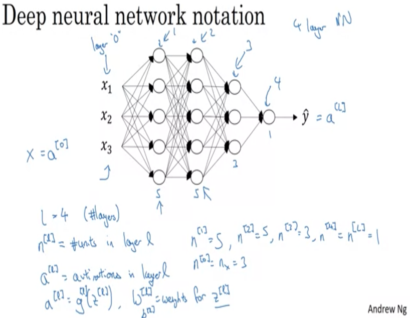
Deep Neural Networks
A Deep Neural Network consists of multiple hidden layers. A neural network with more than one hidden layer is consider deep.
Deep neural networks, which have many layers, have been shown to be more powerful and effective than shallow neural networks, which have fewer layers, for many tasks such as image and speech recognition.
Deep networks are able to learn hierarchical representations of the data, where lower layers learn simple patterns and higher layers learn increasingly complex and abstract patterns based on the outputs of the lower layers.
Additionally, deep networks can be trained more efficiently using techniques such as backpropagation and batch normalization, which helps to improve the performance of the network.
Appendix
Binary Classification
In a binary classification problem, the result is a discrete value output. For example - account hacked (1) or not hacked (0) - a tumor malign (1) or benign(0)
Example: Cat vs Non-Cat
The goal is to train a classifier for which the input is an image represented by a feature vector, 𝑥, and predicts whether thecorresponding label𝑦is 1 or 0. In this case, whether this is a cat image(1)or a non-cat image (0).

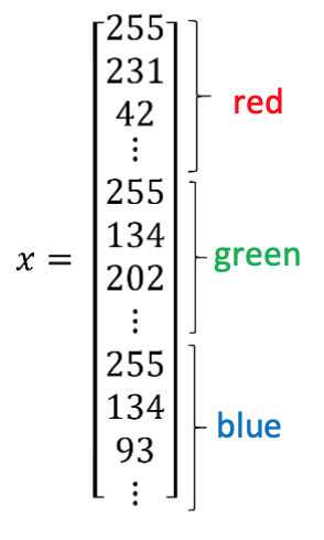
An image is stored in the computer in three separate matrices corresponding to the Red, Green, and Blue color channels of the image. The three matrices have the same size as the image, for example, the resolutionof the cat image is 64 pixels X 64 pixels, the three matrices (RGB) are 64 X 64 each.
The value in a cell represents the pixel intensity which will be used to create a feature vector of n- dimension. In pattern recognition and machine learning, a feature vector represents an image, Then the classifier’s job is to determine whether it contain a picture of a cat or not.
To create a feature vector, 𝑥, the pixel intensity values will be “ unrolled” or “ reshaped” for each color. The dimension of the input feature vector𝑥 is𝑛 = 64𝑥 64𝑥 3 = 12288.
Logistic Regression
Logistic regression is a learning algorithm used in a supervised learning problem when the output 𝑦 are all either zero or one. The goal of logistic regression is to minimize the error between its predictions and training data. Example: Cat vs No - cat
Given an image represented by a feature vector 𝑥, the algorithm will evaluate the probability of a cat being in that image.
𝐺𝑖𝑣𝑒𝑛𝑥, 𝑦̂=𝑃(𝑦=1|𝑥),where 0 ≤𝑦̂≤1
The parameters used in Logistic regression are:
- The input features vector:
𝑥 ∈ R𝑛𝑥 , where 𝑛𝑥 is the number of features - The training label:
𝑦 ∈ 0,1 - The weights:
𝑤 ∈ R𝑛𝑥, where 𝑛𝑥 is the number of features - The threshold:
𝑏 ∈ R - The output:
𝑦̂ = 𝜎(𝑤𝑇𝑥 + 𝑏) - Sigmoid function:
s = 𝜎(𝑤𝑇𝑥 + 𝑏) = 𝜎(𝑧)= 1 / 1+𝑒−𝑧
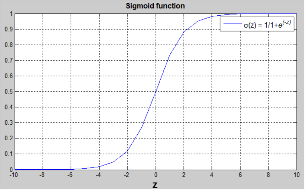
(𝑤𝑇𝑥 + 𝑏) is a linear function (𝑎𝑥 + 𝑏), but since we are looking for a probability constraint between [0,1], the sigmoid function is used. The function is bounded between [0,1] as shown in the graph above.
Some observations from the graph:
If 𝑧 is a large positive number, then 𝜎(𝑧) = 1If 𝑧 is small or large negative number, then 𝜎(𝑧) = 0If 𝑧=0,then 𝜎(𝑧)=0.5
Quiz Answers